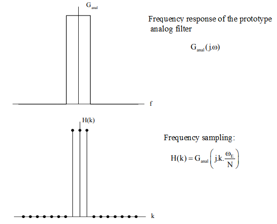
Frequency sampling
We choose to sample at an analogueue frequency where we have the frequency response of the prototype analogueue filter \(G_{anal}(j\omega)\). Therefore, we define the following :
\(H\left(k\right)=G_{anal}\left(jk\frac{\omega_e}{N}\right)\\) (10)
Where N is the number of samples. Using the same example as previously, N = 17, H(0)=H(-1)= H(1)=1 et H(2)=H(-2)= ... =H(8)=H(-8)=0.
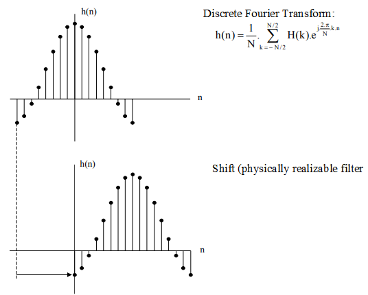
We can deduce, through discrete Fourier transformation (DFT), the values of the impulse response:
\(h(n)=\frac{1}{N}\sum_{k=-\frac{N}{2}}^{\frac{N}{2}}{H\left(k\right)e^{j\frac{2\pi}{N}kn}\ }\) (11)
In our case :
\(h\left(n\right)=\frac{1}{17}\left(1+{It\ is}^{-j\frac{2\ p}{17}n}+{It\ is}^{j\frac{2\ p}{17}n}\right)=\frac{1}{17}\left(1+2cos(\frac{2\ p}{17}n)\right)\) with \(-8≤ n ≤ 8\).
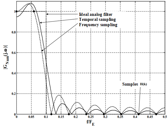
Finally, to make this filter physically realisable, we shift this impulse response by 8 samples. The following page summarizes all these operations. The figure below displays the frequency response of each filter.
Example : Example :
Synthesis of an “ideal” low-pass filter \left(F_C=\frac{F_E}{10}\right): frequency sampling