Chapitre 5

Consider a signal x(t), whose Fourier transform is X(f). We call the Hilbert transform of this signal the signal defined by the relation:

So let x(t) be a signal with Fourier transform X(f). The Hilbert transform of this signal is defined by the relation:

\(\hat{x}\left(t\right)=\frac{1}{\pi}\int_{-\infty}^{+\infty}\frac{x(\tau)}{t-\tau}d\tau\) Ou encore \(\hat{x}(t)=x\left(t\right)\ast\frac{1}{\pi t}\ \ \ \ \ \ \ \ \ \ (32)\)

To understand this integral in strict mathematical terms, consider the Cauchy principal value:

\(\hat{x}\left(t\right)=\frac{1}{\pi}{lim}_{\in\rightarrow0}{\left\{\int_{+\in}^{+\infty}\frac{x(u)}{t-u}du+\int_{-\infty}^{+\infty}\frac{x(u)}{t-u}du\right\}}\) (33)

Since a convolution operator governs this transformation, we can interpret it as linear and time-invariant filtering (Hilbert filter).

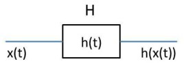
The impulse response of a Hilbert filter is therefore:

\(h\left(t\right)=\frac{1}{\pi t}\) (34)

Note:

Since the function h\left(t\right) is non-causal, the Hilbert filter itself is non-causal and therefore unrealizable (in practice, approximations are made over limited frequency bands). We will assume that the transfer function is:

\(H\left(f\right)=TF\left\{\frac{1}{\pi t}\right\}=-j.sgn(f)\) (35)

with :

\(\begin{matrix}sgn\left(f\right)=-1\ \ \ \ \ \ \ f<0\\sgn\left(f\right)=+1\ \ \ \ \ \ f>0\\\end{matrix}\)

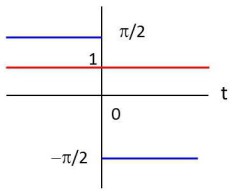
The figure (7) depicts the magnitude of \(\left|H(f)\right|\) in red and the phase in blue. Referring to \(\hat{X}(f)\) the Fourier transform of the Hilbert transform :

\(\hat{X}(f)=TF\left\{\hat{x}(t)\right\}\)

We have :

\(\hat{x}(t)=x\left(t\right)\ast\frac{1}{\pi t}\) \(\xrightarrow{TF}\) \(\hat{X}\left(f\right)=-j.sgn\left(f\right).X(f)\) (36)

Often, one can obtain\( \hat{x}(t)\) from the inverse Fourier transform of \(\hat{X}\left(f\right)\).