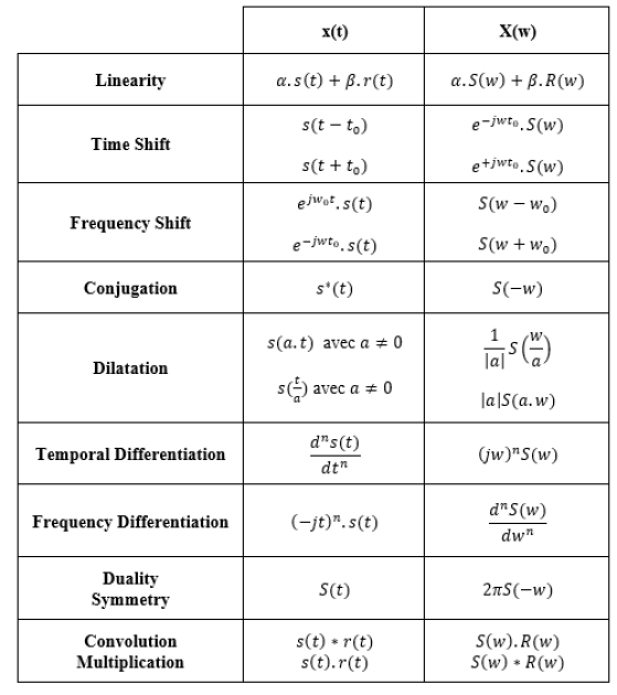
Properties of the Transfer Function (TF)
Consider the two analogous signals: s(t) and r(t).
Fourier transformation of usual signals (refer to Appendix B).
Special case : Dirac Fourier Transform
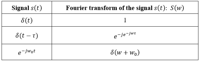
Example :
Application :
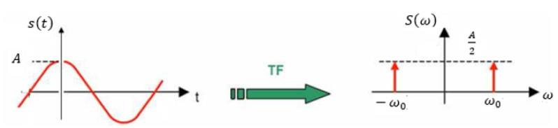
Calculate and illustrate the Fourier transform of a sinusoidal signal s(t) with amplitude S and frequency f0 , given by \(s\left(t\right)=Acos\left(\omega_0t\right)\) , utilising Fourier properties.
Correction :
\(s\left(t\right)=Acos\left(\omega_0t\right)=A\left(\frac{e^{j\omega_0t}+e^{-j\omega_0t}}{2}\right)\)\( \implies\) \(S\left(\omega\right)=\frac{A}{2}\delta\left(\omega-\omega_0\right)+\frac{A}{2}\delta\left(\omega+\omega_0\right)\)
Note :
The Fourier transform of a cosine function of frequency f0 and of amplitude S, is the sum of two Dirac pulses centred on the frequencies -f0 and +f0 ; each with an amplitude half that of the signal: S/2.
The Fourier transform of a sine function of frequency f0 and of amplitude S, and the sum of two Dirac pulses centred on the frequencies -f0 with an amplitude of S/2 and +f0 with an amplitude –S/2.