Autoregressive (AR) models
The AR process is autoregressive.
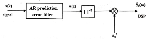
It is assumed that the signal whose PSD we want to estimate represents the output of noise centered through an autoregressive linear filter, as described in Figure 5.
Concretely, if we consider a stationary process x(k), we consider that it is autoregressive of order p if we can explain its value at time k using its previous p terms.
Mathematically, this means that:
\(\forall\ t:x(k)=\sum_{1}^{p}{a_ix(k-i)+\epsilon_k}\) (35)
The noise \(\epsilon_k\) being white with power \(\sigma_u^2\) and (𝛼1, ..., 𝛼p) of the real numbers.
We obtain a Z response from the filter equal to:
\(H(Z)=\frac{1}{\sum_{i=0}^{p}{a_iZ^{-i}}}=\frac{1}{A(Z)} ; a_0=1\) (36)
And the signal's autocorrelation function, which admits a Z transform, is equal to:
\(R_x(Z)=X(Z)X(Z^{-1})=\sigma_u^2\left|H(Z)\right|^2\) (37)
We assume the filter \(H(Z)\) to be stable.
The signal's autocorrelation function is equal to the nearest \(\sigma_u^2\) factor to the filter's.
By changing the variable \(Z\) \(\rightarrow\) \(\omega\) of the relation (37), we obtain the PSD of the signal:
\(\gamma_x(\omega)=R_x\left[e^{j\omega}\right]=\frac{\sigma_u^2}{\left|\sum_{i=0}^{p}{a_ie^{-j\omega i}}\right|^2}\) (38)
We would have estimated the AR coefficients of the filter and the power of the input noise using algorithms like Levinson or Kalman AR.