Estimate Variance
The variance is equal to,
\(\sigma_E^\mathrm{2}=E\left\{\left(\hat{M}-m\right)^\mathrm{2}\right\}=E\left\{{\hat{M}}^\mathrm{2}\right\}-m^\mathrm{2}\) (8)
calculation of de E\(\left\{{\hat{M}}^\mathrm{2}\right\}\)
\(E\left\{{\hat{M}}^\mathrm{2}\right\}=E\left\{\frac{\mathrm{1}}{T^\mathrm{2}}\int_{\mathrm{0}}^{T}\int_{\mathrm{0}}^{T}x\left(t\right)x\left(u\right)dtdu\right\}=\frac{\mathrm{1} }{T^\mathrm{2}}\int_{\mathrm{0}}^{T}\int_{\mathrm{0}}^{T}E\left\{x\left(t\right)x\left(u\right)\right\}dtdu\)
\(=\int_{\mathrm{0}}^{T}\int_{\mathrm{0}}^{T}{E\left\{x\left(t\right)x\left(u\right)\right\}dtdu=\frac{\mathrm{1} }{T^\mathrm{2}}}\int_{\mathrm{0}}^{T}\int_{\mathrm{0}}^{T}{R_xdtdu}\) (9)
By changing the variable:
\(\left[\begin{matrix}t\\u\\\end{matrix}\right]\rightarrow τ=t-uv=u\)
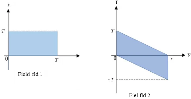
The transformation of the integration domain D1 into the domain D2 (Figure 2) results in the following moment of order:
\(E\left\{{\hat{M}}^2\right\}=\frac{1}{T^2}\left[\int_{\mathrm{-T}}^{0}{\left(T+\tau\right)R_x\left(\tau\right)d\tau+\int_{0}^{T}{\left(T+\tau\right)R_x\left(\tau\right)d\tau}}\right]\)
\(=\frac{1}{T}\int_{-T}^{+T}\left(1-\frac{\left|\tau\right|}{T}\right)R_x\left(\tau\right)d\tau\) (10)
Which gives a variance equal to:
\(\sigma_E^2=\frac{1}{T}\int_{-T}^{+T}\left(1-\frac{\left|\tau\right|}{T}\right)\left[R_x\left(\tau\right)-m^2\right]d\tau\) (11)
So, the estimation variance is the average of the center-adjusted autocorrelation function \(R_{xc}\left(\tau\right)=R_x\left(\tau\right)-m^2\) weighted by the triangle function over the time range \(\left[-T,\ +T\right]\).
As;
\(\sigma_E^2\le\frac{1}{T}\int_{-\infty}^{+\infty}{R_x\left(\tau\right)d\tau}\le\frac{1}{T}\int_{-\infty}^{+\infty}{R_{xc}\left(\tau\right)d\tau}=\frac{\gamma_{xc\ (0)}}{T}\) (12)
When the support T of the realization increases, the variance tends to zero. \hat{M} is therefore a consistent estimator.