Discrete Fourier Transform (DFT)
Limit the duration of x(n), i.e, consider a finite number N of time points.
Discretize the frequency (consider a finite number L of frequency points).
Let {x(0), x(1), ..., x(N − 1)} be a discrete signal of finite duration N. Its DTFT is :
\(X\left(f\right)=\sum_{0}^{N-1}{x\left(n\right)e^{-j2\pi fn}}\) (14)
The discretization of the frequency onL points : \(X(f)\) is periodic with period 1, therefore : \(f=k∆f\) with \(∆f=1L\) . Consequently, the discrete approximation of the DTFT (\(f=\frac{k}{L}\)) of this signal is :
\(X\left(\frac{k}{L}\right)=\sum_{n=0}^{N-1}{x(n)e^{-j2\pi\frac{k}{L}n}}\) (15)
n is the time variable, taking values from 0 to N-1 and k is the frequency variable, ranging from 0 to L-1. In notation: X(k/L)=X(k), where k takes values from 0 to L-1.
Definition :
The DFT, evaluated at L frequency points for a discrete signal, is defined as follows :
\(X\left(k\right)=\sum_{n=0}^{N-1}{x(n)e^{-j2\pi\frac{k}{L}n}}\) (16)
N: number of time points.
n: time variable n = 0, ..., N-1.
L: Number of frequency points.
k: frequency variable k = 0, ..., L-1.
X(k)is periodic with period L.
Note : Noticed :
x̃(n) is a periodic sequence with a period of L.
The discretization of \(X\left(k\right)\) resulted in the periodization of \(x(n)\).
In the following, we will consider L = N.
As observed with the DTFT that: Temporal discretization⇒ frequency periodization
Now with the DFT:
Frequency discretization⇒ Periodization in time
Example: Consider the signal x(n)= 1 for n = 0 and n= 3 and 0 elsewhere.
First, let's calculate the DTFT, which provides :
\(X_e\left(k\right)=\sum_{-\infty}^{+\infty}{x(nT_e)e^{-j2\pi fn T_e}}\) (17)
\(1+e^{-j2\pi fn T_e}=2.\cos(3\pi T_e)e^{-j3\pi f T_e}\) (18)
Now, let's calculate the DFT using N=4 samples (4 samples of the DFT from 4 samples of the signal).
\(X\left(k\right)=\sum_{n=0}^{N-1}{x(n)e^{-j2\pi\frac{k}{4}n}}\) (19)
\(X\left(k\right)=\sum_{n=0}^{3}{x\left(n\right)e^{-j2\pi\frac{k}{4}n}}\)
\(\quad\quad\quad=\left(\begin{matrix}x\left(0\right)\\\begin{matrix}x\left(1\right)\\\begin{matrix}x\left(2\right)\\x\left(3\right)\\\end{matrix}\\\end{matrix}\\\end{matrix}\right)\)
\(X\left(k\right)=\left\{\begin{matrix}x\left(0\right)+x\left(1\right)+x\left(2\right)+x\left(3\right)=\ \ \ \ \ \ \ 2\\x\left(0\right)+x\left(1\right)e^{-j\frac{\pi}{2}}+x\left(2\right)e^{-j\frac{2\pi}{2}}+x\left(3\right)e^{-j\frac{3\pi}{2}}=2.\cos(3\frac{\pi}{4})e^{-j\frac{3\pi}{4}}\\\begin{matrix}x\left(0\right)+x\left(1\right)e^{-j\pi}+x\left(2\right)e^{-j2\pi}+x\left(3\right)e^{-j3\pi}=2.\cos(3\frac{\pi}{2})e^{-j\frac{3\pi}{2}}\\x\left(0\right)+x\left(1\right)e^{-j\frac{3\pi}{2}}+x\left(2\right)e^{-j3\pi}+x\left(3\right)e^{-j\frac{9\pi}{2}}=2.\cos(9\frac{\pi}{4})e^{-j\frac{9\pi}{4}}\\\end{matrix}\\\end{matrix}\right.\) (20)
The magnitudes of the 4 samples of \(X(k)\) are: 2,\(\sqrt2\),0,\(\ \sqrt2\)
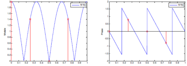
The DTFT curve (in blue) overlays the four DFT samples (in red). This demonstrates that the DFT represents only the sampling of the DTFT within the range of N. It is also noted that the frequency precision is ∆f=fe ⁄ N. We should reduce the frequency step to improve this precision.
DTF of a periodic signal (see Appendix C)
Consider xp (n), a periodic signal with a period of N.
To compute its DTF, we confine our analysis to a single period of N.
DFT Equation : \(X_p(k)\ =\sum_{n=0}^{N-1}{x_p(n)\ e^{-j2\pi\frac{k}{L}n}}\)
The reverse DFT : \(x_p(n)\ =\sum_{n=0}^{N-1}{X_p(k)\ e^{+j2\pi\frac{k}{L}n}}\)
And x(n) is a periodic sequence of period N, x(n) coincides exactly with xp (n). This is not the case for any signal!