Chaptre 1

Various steps and operations are involved in the convolution product:

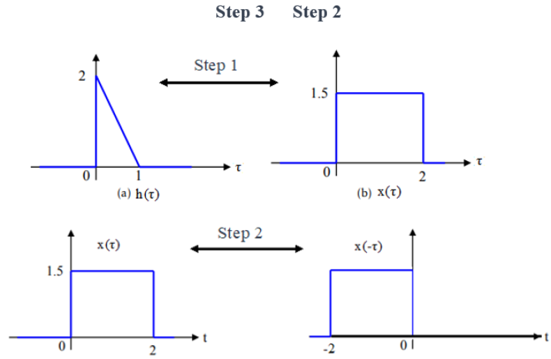
1. The variable t is replaced by τ.

2. We consider the symmetry of f2(t) relative to the ordinate axis f₂ (t) → f₂ (-t).

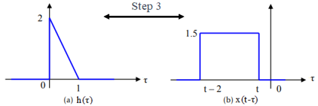
3. The function f₂ (-τ) is then translated to the right by an amount t: f₂ (-τ) → f₂ (t- τ).

4. The product f₁(t).f₂ (t- τ) are computed.

5. The convolution product, being a function of time t, needs to be evaluated over -∞ < t < +∞.

Example : Consider the two functions h(t) = −2t + 2 for 0 ≤ t ≤ 1 and x(t) = 1.5 for 0 ≤ t ≤ 2.

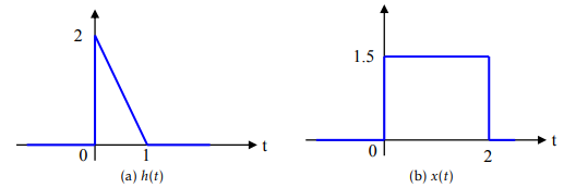
• Calculate: y(t)= h(t)* x(t).

"4th and 5th step "

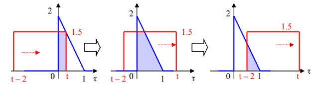
The calculation of the convolution is then done at intervals.

1st case : \(0 < t < 2 \implies\) \(y\left(t\right)=\int_{-\infty}^{+\infty}{h\left(\tau\right)x\left(t-\tau\right)d\tau=}\int_{0}^{t}{(-2\tau+2)(1.5)d\tau}\)

\(y\left(t\right)=3t-1.5t^2\)

2nd case : \(1 < t < 2 \implies\) \(y\left(t\right)=\int_{0}^{1}{\left(-2\tau+2\right)\left(1.5\right)d\tau=1.5}\)

3rd case : \(t > 2 \implies\) \(y\left(t\right)=\int_{t-2}^{1}{\left(-2\tau+2\right)\left(1.5\right)d\tau=1.5t^2-9t+13.5}\)

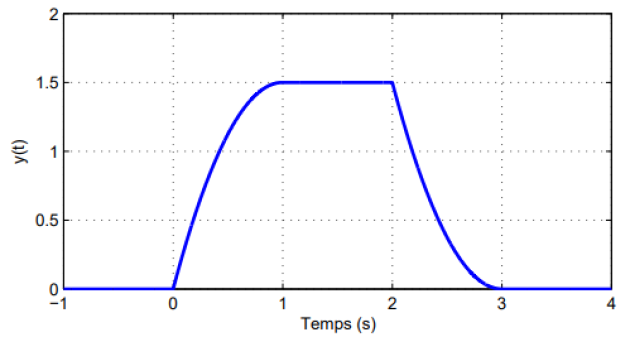
We can validate the derived equations, as the convolution yields a graph without discontinuities. The visual representation of the final result is provided in the figure below.